
Research Article | DOI: https://doi.org/10.58489/2836-5836/012
*Corresponding Author: Chao Wang
Citation: Chao Wang, Yixin Ren, Meiyu Shen, and Yi Tsong. (2024). A Reference Scaled Difference in Means Approach to Equivalence Test for Binary Clinical Outcomes. Clinical Trials and Bioavailability Research. 3(1); DOI: 10.58489/2836-5836/012
Copyright: © 2024 Chao Wang, this is an open-access article distributed under the Creative Commons Attribution License, which permits unrestricted use, distribution, and reproduction in any medium, provided the original work is properly cited.
Received: 16 February 2024 | Accepted: 11 March 2024 | Published: 22 March 2024
Keywords: equivalence test, binary response, variable margin, reference-scaled test, Wald test.
A proposed generic drug product needs to be compared with some reference product through equivalence test to support marketing approval. One important type of treatment outcome is the binary response indicating whether a favorable outcome is achieved. The binary response rates of the test and reference treatments are often compared via their difference with some margin. While the difference can usually be estimated in a clinical study, it is frequently difficult to determine a proper margin. Existing approaches suggest a fixed margin or a margin as a function of the reference response rate, such as step-wise constant margin, piece-wise smooth margin, etc. The issues with existing margin choices were discussed recently and a variable margin was proposed for non-inferiority test, which is a constant multiple of the standard deviation of reference response rate. In this paper, we extended the discussion to equivalence test, which can be formulated as two one-sided tests. Our discussion revealed some unique features of the equivalence test for binary responses with a variable margin. For instance, this approach may improve power control when the reference product has a high response rate. On the other hand, when both sample size and margin multiplier is small, the rejection rate of the equivalence test is nearly zero.
In clinical trials, one important type of treatment outcome is binary response indicating whether a subject has a favorable outcome or unfavorable outcome, often conveniently denoted by 1 and 0 respectively. Let PT and PR be the binary response rates of the test and reference products respectively. For a new test drug proposed as a generic to a marketed reference product, one of the critical requirements for regulatory approval is to establish the equivalence between PT and PR, which is often assessed via some form of equivalence test.
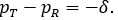
A common form of equivalence test is focused on the difference between the two response rates and is formulated as below,

where δ > 0 is referred to as the equivalence margin.
The equivalence test can also be reformulated as the following two one-sided tests (TOST),

and

The hypothesis test in Eq. (2) is often presented as a non-inferiority (NI) test. An FDA guidance for industry recommends that the NI test be performed with a test size of 2.5% when it is used to establish effectiveness (FDA, 2016). For the case of equivalence test, it is generally accepted that both null hypotheses H10 and H20 be rejected at the type I error rate of 5% to achieve an overall 5% test size.
Regulatory authorities may predetermine a fixed constant margin δ for a particular drug product or a category of drug products. An FDA guidance for industry (FDA, 2003) recommends that bioequivalence be established with clinical endpoints for drugs with low absorption in blood system. A clinical trial of generic drug bioequivalence assessment typically consists of three arms, i.e., placebo (B), test (T), and reference (R) treatments. The investigator needs to compare test with placebo for efficacy, using the following hypotheses,

and to compare reference with placebo to show validation in the study population with the following hypotheses,

Both null hypotheses should be rejected with 2.5% type I error rate before testing for bioequivalence with the hypotheses in Eq (2) and (3) with δ =0.2.
This fixed margin can lead to some difficulties. The variance of the sample response rate is a function of the response rate. Therefore, when the response rate is close to 0 or 1, the variance is smaller, and the equivalence test enjoys a higher power than the case when the response rate is close to 0.5. In fact, the sample size required with a fixed margin can increase up to a magnitude of 2.7 when the true response rates vary from 0.1 or 0.9 to 0.5, assuming equal response rates and equal sample sizes for test and reference treatments (see Eq. 4.2.4 (Chow, Wang, and Shao, Chow et al.)). In addition, Yuan et al. (2018) discussed the power and sample size determination in bioequivalence test of binary endpoints in generic drug applications with a fixed margin of δ =20%, using the same sample size, for the same size of difference, PT and PR, and showed that the power of bioequivalence test depends heavily on the reference response rate. It is of interest to drug developers to
keep sample sizes small to reduce cost and also to regulatory authorities as not to increase unnecessary burden to drug developers. It may be impractical to calculate sample size needed by assuming the worst-case scenario of both response rates equal to 0.5.
In a recent discussion (Ren et al., 2019) for NI test, several common margin choices were compared, such as fixed margin (Tsong, 2007; FDA, 2016), variable margins which are functions of PR, i.e., δ = δ(PR), including step-wise constant margin (FDA, 1992; Röhmel, 1998), and smooth margins (Röhmel, 2001). It was also noted that the reference response rate in the smooth margin was considered to be deterministic by Röhmel (2001). In addition, there was also a comprehensive discussion for NI test with a variable margin (Zhang, 2006).
Step-wise constant margins have also been used in recent studies. To design a proper immunogenicity study of an insulin biosimilar drug product, a constant margin determined by a step function with a maximum sample size of 500 patients was used in Wang (2018), which is reproduced in Table 1.
Table 1: A step function to determine margin, reproduced from Wang (2018).
| ADA Rate of Reference Product (%) | Margin (%) |
| 5 | 5.70 |
| 10 | 7.90 |
| 15 | 9.30 |
| 20 | 10.50 |
| 25 | 11.30 |
| 30 | 12.00 |
| 35 | 12.50 |
| 40 | 12.80 |
| 45 | 13.00 |
| 50 | 13.10 |
| 55 | 13.00 |
| 60 | 12.80 |
In this paper, we extend the smooth variable margin originally proposed for NI test (Ren et al., 2019) to the two-sided equivalence test. Although there are some similarities between the equivalence test and NI test, we found some features unseen for the case of the one-sided NI test. For instance, the rejection rate of the equivalence test is nearly zero when both sample size and margin multiplier is small, regardless the values of PT and PR.
The paper is organized as follows. A formal discussion of the problem and test statistics are presented in Section 2. Section 3 reports simulation studies. Section 4 concludes the paper with additional discussion. More technical details are deferred to the Appendix.
FDA recommends to use the reference scaled average bioequivalence test for products with large variability (FDA, 2001, 2011; Tothfalusi and Endrenyi, 2016). The test can be stated as below,

where μT and μR are are the means of test and reference respectively; σR is the standard deviation of reference product; δ is the pre-specified equivalence margin. This hypothesis can also be presented as follow,

For binary data, the test can be presented as follow,

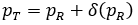
where PT and PR are the response rates of test and reference respectively; δ = δ(PR) is the equivalence margin represented by

Test statistics

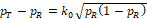
In the following discussion, we use the margin function originally proposed by (Ren et al., 2019), which is a multiple of the standard deviation of sample estimate for PR,

where k > 0 is referred to as the margin multiplier, the selection of which will be discussed later.
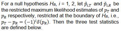
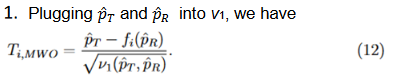
We consider the following Wald type test statistics for equivalence test,
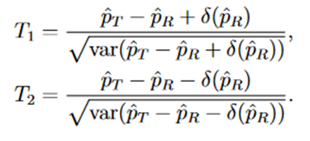
Let

then T1 and T2 can be written as follows,

Three methods for calculating the variances,
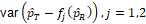
, were discussed
and compared based on asymptotic normal approximation previously (Ren et al., 2019). For the purpose of benchmarking the performance, the same methods are used here.
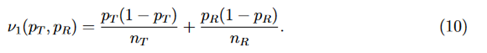
The first method ignores the margin variability, which gives a naive version of the variance and is frequently used in practice,
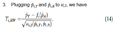
The second and third methods take into account the margin variability but differ in the response rates at which they are evaluated. Since

, by the delta method, it follows that

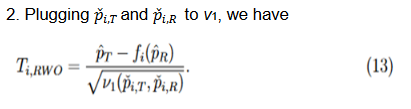
Both

and

were shown to control type I error considerably inferior to

for NI test (Ren et al., 2019). This is also true for

and

compared with

for equivalence test, which can be seen in the simulation studies reported later in this paper. Thus, only the power function of

is considered here.
Assume that there exist some

and

such that

and

in probability. Further assume that
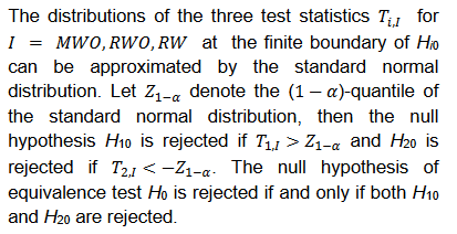
. Then the approximate power functions can be given as below (more details can be found in the Appendix),
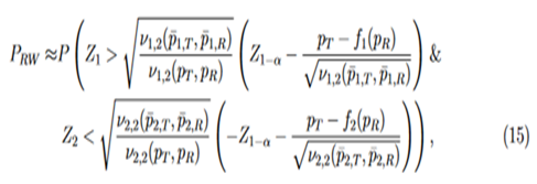
where

j = 1,2, and (Z1 and Z2) is a random vector with an asymptotic bivariate normal distribution, each following the standard normal distribution with asymptotic correlation given by
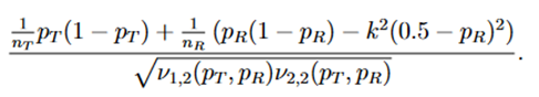
Then the power function can be given approximately by the probability of a bivariate normal distribution over a region defined by Eq. (15), which can be calculated numerically by the pmvnorm function in the R package mvtnorm (Genz et al., 2018; Genz and Bretz, 2009).
Two methods can be used to determine k based on the sample size of the study (Ren et al., 2019). The first method is intended to be used for large sample studies, and the second for small sample studies. First, we note that for a constant k, when

then

, and thus H10 is always rejected since

is a probability. Similarly, if

, then
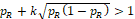
, and thus H20 is always rejected.
For studies with large sample sizes, k may be selected so that the variable margin is similar to margins used in previous studies. As an example, for the biosimilar immunogenicity trial of insulin product in Wang (2018), which has at least 250 per arm, we match the step-function margin with our variable margin at PR = 0.5,
Solving Eq. (16) for k, then we have k = 0.262 and margin function
. In fact, the margin function agrees with the step function at the thresholds.For small sample studies, setting k = 0.262 may render the test of little power. Simulation studies reported below showed that when

the equivalence test cannot reject Ho for any combination of PT and PR. However, there are practical situations where it is impractical to obtain relevant large sample sizes, while sufficient power is still needed. In this regard, one may choose k for a test statistic by setting the power function in Eq. (15) to be

and solve for k for some presumed PT and PR. The solved k is implicitly also a function of PT, PR and the sample sizes. To facilitate the discussion, we consider the case when both test and reference response rates are the same, i.e.,

, so that the equivalence test has the maximum power, and the sample sizes

For the power function in Eq (15), the main difficulty lies in the unknown

and

and their dependency with k. Because no explicit formulas of

and

are available, we estimate it by bootstrap for any given k. Then k is solved by the R function uniroot in the stats package (R Core Team, 2017).
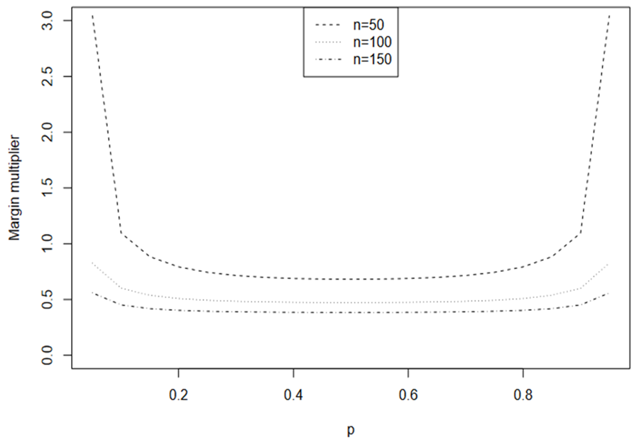
Assuming α = 0.05, β = 0.1, i.e., 90% power, and n = 50, 100, 150, the calculated margin multipliers for

are illustrated in Fig. 1. Except when P is very small, the margin multiplier k seems to be symmetric at

and an increasing function with respect to

. Note that when n = 50, very large k is required to obtain the prespecified power. A large k can result in trivial lower bound

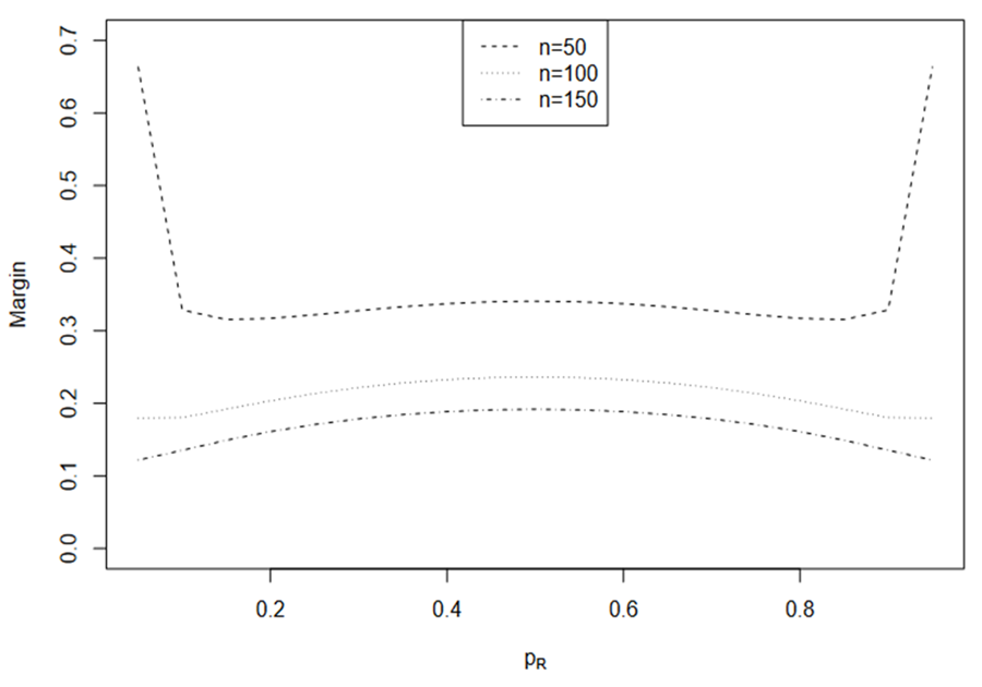
or upper bound

and this is more often as k increases. The induced margins are shown in Fig. 2. Interestingly, the induced margin curves are rather flat for a given sample size except when PR is close to 0 or 1. For n = 50, the margin ranges from 0.315 to 0.341, excluding the margins for PR = 0.05 and PR = 0.95. The margin ranges from 0.18 to 0.236 for n = 100 and from 0.122 to 0.192 for n = 150.
Empirical type I error
Here we report a simulation study of the empirical type I error of the three test statistics in large sample studies with k = 0.262. We assume equal sample size for both arms, and consider a variety of sample sizes, nT = nR = 50, 100, …, 500 and the true reference probability

For each PR, the margin and true PT, are given by

respectively. For given sample size and true response rates, the test and reference data are simulated by

Three equivalence tests based on test statistics

are performed for each simulated sample at a nominal level of α = 0.15.The simulation study is replicated for 10^6 times.
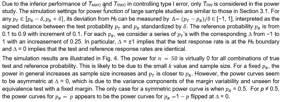
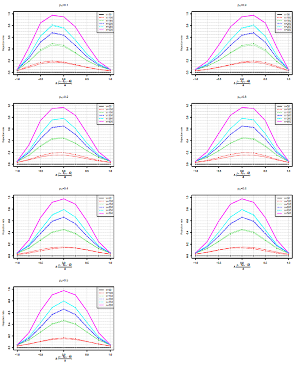
The performances of the three tests are similar when sample sizes changes, so only empirical rejection rates (ERR) (type I errors) for
and theoretical rejection rates (TRR) for TRW are reported in Figure 3 for the case when

When sample size is 50, all tests have almost zero rejection rate, regardless the true reference probability. This is due to the small sample size and the small k value. When sample size is 100, the rejection rates are around 0.03. Note that the theoretical rejection rate for TRW is also close to 0.03. The rejection rates for sample sizes at least 150 are similar across different sample sizes, showing that both TRWO and TMWO have seriously bias in type I error, compared with TRW for which both the empirical type I error and theoretical approximations are much closer to the nominal 0.05 level.
The evident trends in ERR for TRWO and TMWO are mainly due to the variance estimates ignoring the variability in the margin. The uprising trend cross the 0.05 nominal size at PR = 0.5 may be explained below. First note that the simulation study is set at the lower boundary
This is the reason for the comparable rejection rates of TRWO and TMWO. Also, H2,0 is almost always rejected. So the type I error of the equivalence test is close to the rejection rate of H1,0. For this selected k and any

implying T1,RWO < T>1,RW and thus T1,RWO rejects H1,0 less frequently than T1,RW.
Additional simulation study conducted with
.
unreported here shows a mirrored pattern for TMWO and TRWO, of which downward trends were observed for type I error.
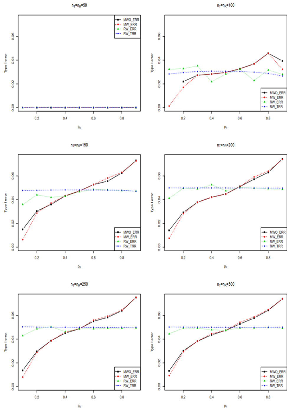
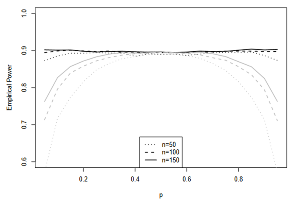
Verification of margin multiplier k for a prespecified power
Here we verify the calculation of margin multiplier k for TRW. The data are simulated with PT = PR = P and n = nT = nR = 50, 100, 150 with P = 0.05, 0.1, …., 0.90. For each n and each P, two sets of simulations are performed. In the first set, the test is performed with the k calculated with a target of 90% power and true P with given n. In the second set, the test is performed with the previously computed k which yields 90% power for,

In this paper we extended the discussion of comparison of binary test and reference responses with a variable margin in the form of reference scaled difference in means from NI test (Ren et al., 2019) to equivalence test. Three test statistics were studied and both theoretical discussion and simulation studies showed that the variability in the margin should be taken into account to construct proper test statistics so TRW is recommended. The type I error of TRW is closer to the nominal size for PR close to 1 than PR close to 0. Our calculation of the margin multiplier showed that when a fixed power is desired, the margin does not vary much as the reference response rate changes. Simulation studies showed that small margin multiplier may result in zero rejection rates so sufficiently large sample size should be maintained to achieve proper control of type I error and desired power as the weakness of two one-sided tests.
For TRW, the power function is
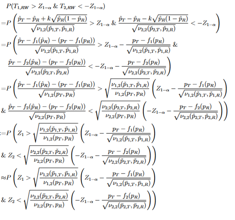
There is no deterministic order between the random variables Z1 and Z2. Both have asymptotic standard normal distribution with asymptotic correlation given by
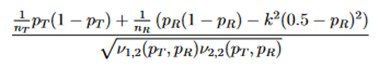
Then the power function can be given approximated by the probability in the last display, which is a probability of a bivariate normal distribution over a region, can be calculated by the function pmvnorm of the R package mvtnorm (Genz et al., 2018; Genz and Bretz, 2009).